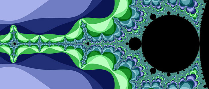
On March the 26th 2012, James Cameron and his submarine craft, Deepsea Challenger, explored the depths of the ocean down to 11km under sea level at 11.329903°N 142.199305°E, an infinitesimal point on the surface of the Earth’s vast Oceans. Could you imagine how incredible it would be to have thousands of “Deep Challengers” reaching the bottom of our planet in parallel? What a map we would get!
|
|
|
|---|
Throughout the lines of this post we’ll see how such a feat is possible, just let me replace the Earth’s Oceans with The Mandelbrot Set and thousands of “Deepsea Challengers” by Hundreds of distributed execution units. Yes! We will see how it is possible to draw HUGE 2D representations of this beautiful fractal using the distributed computational power which only Apache Spark can provide.
What is this fractal about?
As the reader surely knows, fractals are self-repetitive physical or abstract structures such as geometric figures generated by repeating their dominant features as they get zoomed in on.
The Mandelbrot set is a set of complex numbers whose 2D representation shows the self-replication property of fractals. This representation consist of drawing the points belonging to the complex set in a 2D plane using a given color, let’s use black, and the points not on the set with a different color, we’ll see which one (or rather which color palette) soon.
Drawing figures with complex numbers
2D complex number representation is as simple as using the real part as the value for the x-axis value and the imaginary part as a value in the y-axis. e.g: The complex value -1+2i could be represented as:

Thus a set of infinite points cover a surface, potentially forming a geometric figure, e.g:

As we can’t handle an infinite number of points, the resolution of the surface would be given by the number of points in the set, the more you have, the less porous the painted surface is.
So, yes, it is possible to draw things by just providing a set of complex numbers. And The Mandelbrot set is a complex set, this has been known for ages by now. See this example of a representation created by a primitive computer in 1989:

So it is done, why Spark?
There you go, a single 1989 computer was already able to draw a representation of the set so that’s all, end of the post. I hope you enjoyed it…
Just kidding! The problem with the figure above is that it is so coarse , so zoomed out that you don’t see anything beyond a kind of bug, maybe some kind of Rorschach test , nothing of apparent interest. The ancient computer is to blame in this case. it couldn’t provide a large enough set to represent the nuances of the details hidden behind this black blob. Lets jump 30 years in the future and see what Spark can provide given the same mathematical description:

Hey! those strange branches aren’t a anything else than the figure itself!

This is an improvement for sure! But, believe me, you could have generated this “high resolution” image with a cheap PC in less than a minute. We haven’t discussed the details of the algorithm yet but, I promise you, there is no need to use the power of distributed computation to create this representation.
An infinite universe to explore
The colourful representation shown above is yet small just 1MP (Mega Pixel). However, the points in the complex set are infinite, meaning that you could keep zooming in and calculating whether or not the, each time more infinitesimal, points of the 2D plane fall inside or outside the set. To paint them in black, if they fall inside, or in another color if not. No, there is nothing wrong with your screen nor with your perception (at least regarding this): All of a sudden we have colors! Let’s ignore them and keep in mind that the black dots are those representing complex numbers within the Mandelbrot Set.
A good analogy here are black holes, everything within their event horizon is not there to see: It is black, the information around it is what we can actually see in a colorful fashion.
So, before explaining how, let’s take a look at the result of using distributed computation with Apache Spark to compute a ONE TERAPIXEL REPRESENTATION OF THE MANDELBROT SET.
Don‘t be shy, enter and explore yourself. In any case, you can find an example in the following video:
Is in these extremely huge cases where more computational power is needed, where we can harness the potential of distributed systems to reach levels of detail hardly imaginable for a single computer.
Colors, unveiling the algorithm
So far, we’ve just discussed what this is all about and seen the results of this experiment, now it’s time to start digging right into how this huge, but limited at the same time, snapshot of an infinite universe can be generated.
We can ignore distribution, parallelization and fancy computation accelerators for now and center our attention in the classical sequential algorithm. As we have discussed by now, the idea is to map complex values onto an area on a 2D plane, let’s refer to that rectangular region as our canvas. To map these complex numbers, first we have to find them.
For that, we will sample the 2D plane, that is an interval of complex numbers, and check which elements of the sample fall into the set. A relatively simple algorithm to test whether or not a complex number is part of the set is the Escape Time Algorithm . Without getting into the mathematical details (which are better explained at Wikipedia than by any attempt of me to bring them to this TLDR post) the idea is:
- Take z = 0 as starting value.
- Take as c the complex value whose belonging to the set we want to check.
- Compute the result of the (tail) recursive function:
// Not the actual implementation, a quick draft to illustrate the idea.
def f(z: Complex, c: Complex): Boolean = {
    if(modulus(z) > 4.0) false /* ESCAPED THE RECURSION!
                                  c wasn't part of the set */
    else f(z*z + c)
}
If we run the snippet from above. We have two options: Keep our computer running until the end of the universe or change f to stop iterating at a certain number of iterations. The points in the set are guaranteed to not make z^2+c diverge therefore, by definition, f(Complex.Zero, cInput) should indefinitely call to itself. Thus, the function should be changed to include some kind of limit:
// Not the actual implementation, a quick draft to give you an idea.
def f(z: Complex, c: Complex)(maxIterations: Int): Boolean = {
    if(modulus(z) > 4.0) false /* ESCAPED THE RECURSION!
                                  c wasn't part of the set */
    else if(maxIterations == 0) true
    else f(z*z + c)(maxIterations-1)
}
And this way, we’ve transformed the algorithm into an approximation algorithm where the accuracy of its results increase as the initial limit of iterations increases. That is, the probability of getting false positives (wrongly acknowledging values as belonging to the set) increases as maxIterations gets reduced, sadly for us, the bigger this limit is, the slower the algorithm is.
Having to constraint the number of iterations is a toll we’ve to pay if we want to get our results in a reasonable time. Nevertheless, it has a silver lining, a cool feature which bestows our representation with colourful contours. What if, due to the points not belonging to the set and therefore escaping before reaching the limit, we returned the number of iterations it took to diverge?
// Not the actual implementation, a quick draft to make an idea.
def f(z: Complex, c: Complex)(
    maxIterations: Int,
    currentIteration: Int = 0
): Option[Int] = {
    if(modulus(z) > 4.0) Some(currentIteration)
                               /* ESCAPED THE RECURSION!
                                  c wasn't part of the set, that is now
                                  represented by returning Some(noIterations)
                                */
    else if(currentIteraton == maxIterations) None /* Reached the limit, not interested
                                                      in the number of iterations as
                                                      the function didn't escape */
    else f(z*z + c)(maxIterations, currentIteration+1)
}

val explorationResult: Option[Int] = f(Complex.Zero, Complex(x, y))(1000)
val inMandelbrotSet: Boolean = explorationResult.isEmpty

/* The number of iterations for escaped values can be used
   to give color to the complement set of Mandelbrot set */

val palette: Vector[Color] = ???

val color = explorationResult map { n =>
    palette(n % palette.size)
} getOrElse Black
This algorithm produces nice results for small samples or small limits to the number of iterations, you can find a single threaded implementation which can be run in your very own browser at https://github.com/pfcoperez/mandelbrot_scalajs, it is in this experiment repository as well, implemented without notions of parallelization. We are about to discover that it can be used in a parallel computation just as it is, no changes required:
package org.pfcoperez.iterativegen

object MandelbrotSet {

  /** A single iteration of the numeric method
    *  O(1)
    *
    * @return `None` if the point escapes the set,
    *         `Some(new complex state)` otherwise.
    */
  def iteration(
                 zeroth: (Double, Double)
               )(
                 xy: (Double, Double)
               ): Option[(Double, Double)] = {
    val (x, y) = xy
    val (x0, y0) = zeroth

    if(x*x + y*y >= 4.0) None
    else Some((x*x - y*y + x0, 2.0*x*y+y0))
  }

  /** Several iterations, it can be used to approximate
    *  Mandelbrot's set. The more iterations,the better
    *  the approximation is.
    *
    * O(nIterations)
    *
    * @zeroth Start point, e.g: (x,y) \in ([-2.5, 1], [-1,1]) area.
    * @nIterations Max depth to be check in the recursion.
    * @prevSt Starting point in the expliration
    * @return The state after `nIterations` or condition escape.
    *
    */
  def numericExploration(
                          zeroth: (Double, Double),
                          nIterations: Int,
                          prevSt: Option[((Double, Double), Int)] = None
                        ): (Option[(Double, Double)], Int) = {

    val (prevPoint, prevIterations) = prevSt.getOrElse((0.0, 0.0) -> 0)

    def numericExploration(current: (Double, Double), it: Int): (
      Option[(Double, Double)], Int
      ) =
      if(it == nIterations) (Some(current), prevIterations+it)
      else iteration(zeroth)(current) match {
        case Some(p) => numericExploration(p, it+1)
        case _ => (None, prevIterations+it)
      }

    numericExploration(prevPoint, 0)

  }

}
Explorers Galore!
Coming back to James Cameron’s adventures, given the coordinates of a point on the Earth surface, he explored that point by going deeper and deeper with his submarine. This is exactly what we’re doing with our Escape Time Algorithm, we set a point in our canvas and then we descend as deep as the maximum number of iterations determines:
- We might make a remarkable discovery before reaching the bottom, that is, the point escaped the set before stopping because we reached the maximum number of iterations.
- We might as well reach the bottom empty-handed and assume the point belongs to the set. Remember, this is an approximation algorithm.

Now, consider having a fleet of explorers diving running in parallel. If our goal is to cover the maximum area in the most dense way possible, getting a complete representation would very much help, wouldn’t it?
A dive into the depths is a run of the escape algorithm, we don’t need to make any effort in trying to parallelize the exploration for a single point, we just need to apply it to each element of our sample in a parallel and, even better, distributed way. Spark not only makes this possible but also makes child’s play of it.
The sample is a mess mesh
- Our input is our sample.
- Our sample, a set of 2D points, that is (x,y) values to determine whether or not they represent a complex number belonging to the Mandelbrot Set. That is, a mesh of points covering a 2D region.

The square with x in [0,2] and y in [1,3] is a region sampled by the blue dots {(0,1), (1, 1), (2, 1), (0,2), (1, 2), (2, 2), (0,3), (1, 3), (2, 3)} This set of dots is what we call a mesh. - And our output, coloured images: In black for those points in the set, following a color palette for those that escaped it.
Generating that kind of mesh in Spark is easy. It is just a collection of (x,y) tuples:
- Describe all values for x:
val x = sc.range(0,3,1) //sc <- SparkContext
- Describe all values for y:
val y = sc.range(1,4,1)
- Build a mesh combining both ranges with cartesian product, conveniently provided by Spark as an RDD operation:
val mesh = x cartesian y
Come on! give it a try:
scala> mesh.collect foreach (println)

(0,1)
(0,2)
(0,3)
(1,1)
(1,2)
(1,3)
(2,1)
(2,2)
(2,3)
As our output will be an image, we will be generating our sample as a mesh of pixels by just applying some scaling transformations, it is possible to map those pixels into the complex region we want to explore. If you’re curious about how that was done you can take a look at Primitives2D.scala object. Scaling is performed by taking into account your working context (pixel points or real points). Depending on our selected 2D area, those pixel points will be automatically transformed into real points representing complex values:
...
...
...

case class PixelFrame(upperLeft: Pixel, bottomRight: Pixel) extends Frame[Long]
  case class RealFrame(upperLeft: Point, bottomRight: Point) extends Frame[Double]

  case class Scale(realFrame: RealFrame, pixelFrame: PixelFrame)

  object Implicits {

    implicit def tuple2pixel(t: (Long, Long)): Pixel = {
      val (x, y) = t
      Pixel(x, y)
    }

    implicit def tuple2point(t: (Double, Double)): Point = {
      val (x, y) = t
      Point(x, y)
    }

    implicit def real2pixel(p: Point)(implicit scale: Scale): Pixel = {
      import scale._
      import p._

      require(realFrame contains p, s"$p out of $realFrame")

      val (pxMin, pxMax) = pixelFrame.xRange
      val (pyMin, pyMax) = pixelFrame.yRange

      val (xMin, xMax) = realFrame.xRange
      val (yMin, yMax) = realFrame.yRange

      val px = pxMin + ((pxMax-pxMin)*(x-xMin)/(xMax-xMin)).toLong
      val py = pyMin + ((pyMax-pyMin)*(y-yMin)/(yMax-yMin)).toLong

      Pixel(px, py)
    }

    implicit def pixel2real(p: Pixel)(implicit scale: Scale): Point = {
      import scale._
      import p.{x => px, y => py}

      require(pixelFrame contains p, s"$p out of $pixelFrame")

      val (pxMin, pxMax) = pixelFrame.xRange
      val (pyMin, pyMax) = pixelFrame.yRange

      val (xMin, xMax) = realFrame.xRange
      val (yMin, yMax) = realFrame.yRange

      val x = xMin + (xMax-xMin)*((px.toDouble-pxMin)/(pxMax-pxMin))
      val y = yMin + (yMax-yMin)*((py.toDouble-pyMin)/(pyMax-pyMin))

      Point(x, y)
    }

  }

...
...
...
We could’ve implemented the “scale” concept as a burrito, I mean, a Monad. I didn’t consider that at the time I was hurrying to build the experiment as fast as I could, quite an error as Invariant could have removed all that unnecessary boiler plate.
Mapped out “virtual world”: DONE
Got a map and an army of vehicles, wonders await
At this point we are ready to get a first approximation of the set. We’ve got a collection of points, a sample, in a distributed collection, a RDD[(Long, Long)] it only takes filtering over it using the escape algorithm shown above to know which points should be black, which ones are part of the set:
val (w, h) = dimensions // Resolution, in pixels, of the sample

//sc <- SparkContext
val x = sc.range(0,w,1)
val y = sc.range(0,h,1)

val mesh = x cartesian y

implicit val scale: Scale = Scale( //Select complex interval [-2.5-i, 1+i]
                                   RealFrame(-2.5 -> -1.0, 1.0 -> 1.0),
                                   PixelFrame(0L -> 0L, (w-1L, h-1L))
                                 )

val pointsInMandelbrotSet = mesh filter { (x, y) =>
  val point: Point = Pixel(x, y) //Automatically applies the scale defined above
  val (st, _) = numericExploration(point.tuple, maxIterations)
  st.nonEmpty /* If the end state of the exploration is None,
                it is because it escaped the set, there is no more state to continue iterating. */
}
As easy as that, we distributed the computation in less than twenty lines.
To be continued…
If you’re familiar with how Spark works you might be thinking “Oh boy, that’s an awful lot of shuffling!” and you would be right. If not, you’ll see why that is the case and, in any case, you’ll discover how to avoid that.
See you soon to discuss that and other optimizations, as well as a thorough description of how these distributed collections can become images.


